Tutorial: Bayesian Testing of Central Structures in Psychological Networks
Introduction
This tutorial demonstrates how to use networks (specifically Gaussian graphical models or GGMs) to
- Generate hypotheses
- Perform confirmatory tests on the generated hypotheses
Network theory has emerged as a popular framework for conceptualizing psychological constructs and mental disorders. Initially, network analysis was motivated in part by the thought that it can be used for hypothesis generation. Although the customary approach for network modeling is inherently exploratory, we argue that there is untapped potential for confirmatory hypothesis testing. These ideas are expanded upon in our recent paper, “On Formalizing Theoretical Expectations: Bayesian Testing of Central Structures in Pyschological Networks”, where we merge exploratory and confirmatory hypotheses into a cohesive framework based on Bayesian hypothesis testing. You can find the preprint here.
In what follows, I will describe how you can use R to perform confirmatory hypothesis tests based on initial, exploratory hypotheses with GGMs. For clarity, some code chunks have been omitted, but the full code to reproduce this document can be obtained on the Open Science Framework or GitHub.
Examples
PTSD Network
To begin we need several packages:
BGGM: to conduct exploratory and confirmatory analyses with GGMsMASS: to generate data from covariance matricesnetworktools: to calculate bridge centrality statistics
# Uncomment and run  if missing packages

# for latest version of BGGM
# remotes::install_github('donaldrwilliams/BGGM')

# packages <- c("MASS", "networktools")
# if (!packages %in% installed.packages()) install.packages(packages)
library(MASS)
library(networktools)
library(BGGM)The first dataset contains measurements on 16 PTSD symptoms in 3 communities, “Re-experiencing”, “Avoidance”, and “Arousal” (Sample 4 in Fried et al., 2018). Only the correlations matrices are available so we have to generate the data using MASS::mvrnorm with empirical = TRUE. This ensures that the generated data have the exact covariance structure we give it. The correlation matrix, ptsd_cor4, is loaded with BGGM.
set.seed(1812)

# data for exploratory analyses
explore_ptsd <- mvrnorm(n = 965,
                        mu = rep(0, 16),
                        Sigma = ptsd_cor4,
                        empirical = TRUE)
colnames(explore_ptsd) <- node_names
Exploratory analysis
Estimate graph
The approach begins by estimating an exploratory network. With BGGM, this requires calling the explore function to obtain and sample the posterior distribution. These results are saved in explore_network. The select function takes the results from an explore call, and is used to determine the edge set for \(\mathbf{A}^{CD}\) and \(\mathbf{A}^{CI}\) — the conditional (in)dependence structures. We used type = "continuous" as the data we generated are multivariate normal, but the latest version BGGM can also handle ordinary and binary data.
Note that alternative = "exhaustive" is used for determining the edge set. This returns three adjacency matrices. One for positive, negative, and null edges. In the paper, we focus on positive and null relations. The former is due to the expectation that edges in psychological networks are expected to be positive (i.e., a positive manifold).
# sample posterior distribution
explore_network <- explore(explore_ptsd,
                           type = "continuous",
                           iter = 5000)

# determine edge set
selected_network <- select(explore_network,
                           alternative = "exhaustive",
                           bf_cut = 3)
Bridge Centrality
The next step is to calculate bridge strength using the networktools package. This is similar to node strength, in that, for a given node, it is the sum of the absolute values of its edges. However, bridge strength only takes into account edges that connect to different communities, or clusters. Thus, it is a measure of inter-community connectivity, and can be used to identify central structures in a network.
# retain positive partial correlations from selected network
partial_cors <- selected_network$pcor_mat * selected_network$pos_mat

# rename columns with node names
dimnames(partial_cors) <- list(node_names, node_names)

# calculate bridge strength. comms is a vector specifying
# the community for each node
bridge_strengths <- bridge(partial_cors, communities = comms)$`Bridge Strength`

# we use the top 10% in bridge strength as bridge nodes
bridge_strength_cutoff <- quantile(bridge_strengths, 0.9)
bridge_strengths[bridge_strengths > bridge_strength_cutoff]
## B4 D1
## 0.532 0.657Notice that the partial correlation matrix was multiplied by adjacency matrix for partial correlations (selected_network$pos_mat). This ensures we are only focusing on positive associations.
Calculating bridge strength indicates that nodes B4 and D1 are the top bridge nodes.
Plot bridges
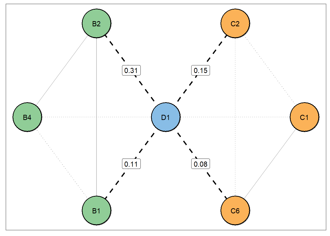
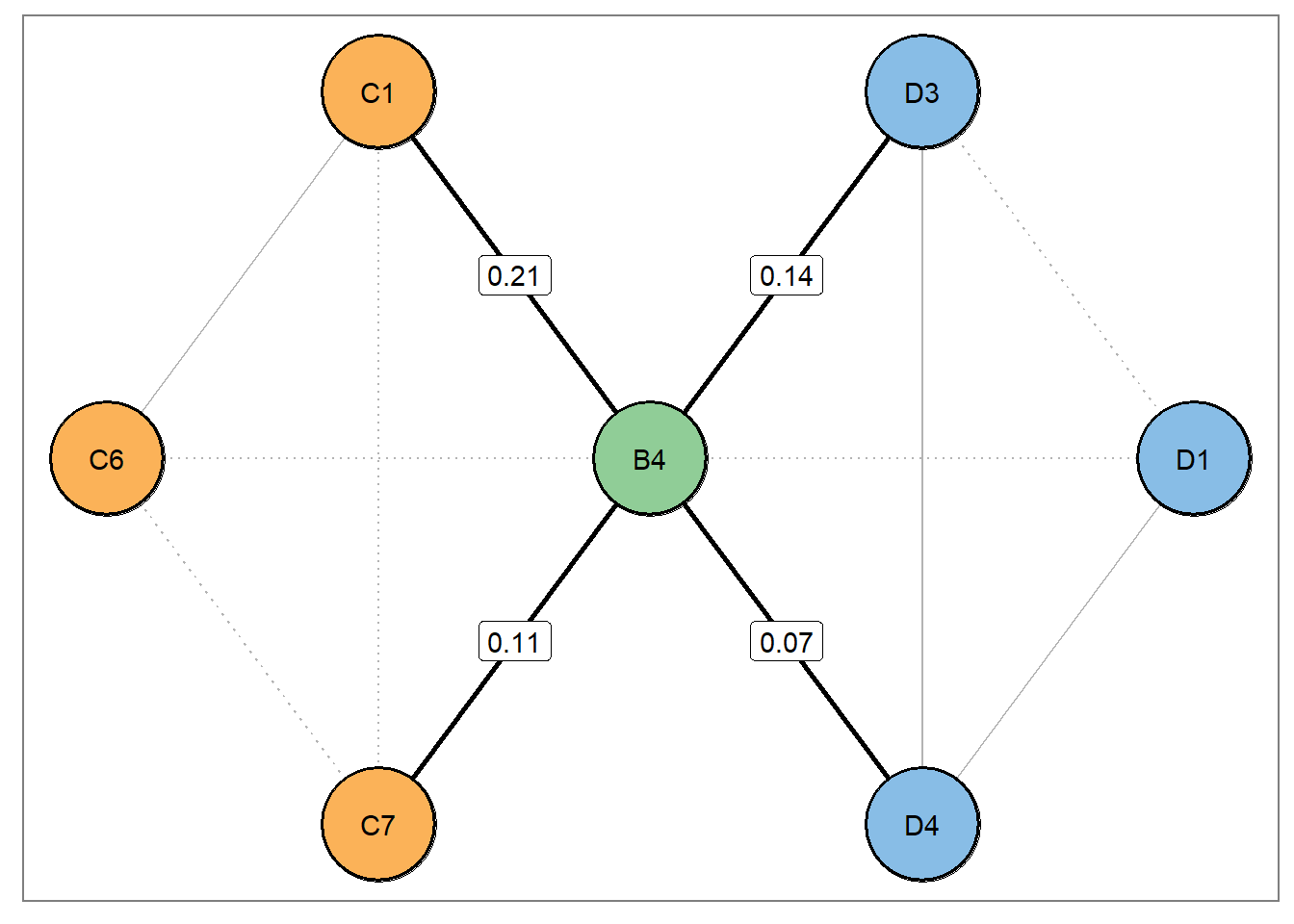
A key idea in our paper was that highlighting and “zooming” in on central structures allows researchers to easily formulate hypotheses. For example, we plotted the neighborhood of bridge relations for nodes D1 and B4.
Confirmatory analysis
With the central structures identified and plotted, we can then move on to formulating and testing hypotheses.
For this confirmatory analysis, data were generated from another correlation matrix (Sample 3 in Fried et al., 2018). This was done to test our hypotheses on a different dataset than the one used for exploratory analysis.
set.seed(1)

confirm_ptsd <- mvrnorm(n = 926,
                        mu = rep(0, 16),
                        Sigma = ptsd_cor3,
                        empirical = TRUE)

colnames(confirm_ptsd) <- node_names
Varying degrees of replication
We first focus on node B4 and test the following hypotheses \[\begin{align} \mathcal{H}_1&: (\rho_{B4-C1}, \rho_{B4-C7}, \rho_{B4-D3}, \rho_{B4-D4}) > 0 \\ \nonumber \mathcal{H}_2&: \rho_{B4-C1} > (\rho_{B4-C7}, \rho_{B4-D3}, \rho_{B4-D4}) > 0 \\ \nonumber \mathcal{H}_3 &: ``\text{not}\; \mathcal{H}_1 \; \text{or}\; \mathcal{H}_2 \text{.''} \end{align}\]
Above, \(\mathcal{H}_1\) is testing for replication of all edges but is otherwise agnostic towards the interplay among bridge relations. \(\mathcal{H}_2\) then provides a refined view into the bridge neighborhood by testing an additional constraint that the strongest edge replicated. That is, all of the bridge relations and the strongest edge re-emerged in an independent dataset. Furthermore, \(\mathcal{H}_1\) and \(\mathcal{H}_2\) both reflect a positive manifold. We also included \(\mathcal{H}_3\) which accounts for structures that are not \(\mathcal{H}_1\) or \(\mathcal{H}_2\).
To test these hypotheses, we can write them out in a single string and use the confirm function. Note that hypotheses are separated by a semicolon, and that partial correlations are denoted as node1 -- node2. The output is obtained by simply printing out the results of confirm.
hyp_var_rep <- c("(B4--C1, B4--C7, B4--D3, B4--D4) > 0;
                   B4--C1 > (B4--C7, B4--D3, B4--D4) > 0")

confirm_var_rep <- confirm(confirm_ptsd,
                           hyp_var_rep,
                           iter = 50000)
confirm_var_rep
## BGGM: Bayesian Gaussian Graphical Models
## Type: continuous
## ---
## Posterior Samples: 50000
## Observations (n): 926
## Variables (p): 16
## Delta: 15
## ---
## Call:
## confirm(Y = confirm_ptsd, hypothesis = hyp_var_rep, iter = 50000)
## ---
## Hypotheses:
##
## H1: (B4--C1,B4--C7,B4--D3,B4--D4)>0
## H2:
## B4--C1>(B4--C7,B4--D3,B4--D4)>0
## H3: complement
## ---
## Posterior prob:
##
## p(H1|data) = 0.197
## p(H2|data) = 0.797
## p(H3|data) = 0.006
## ---
## Bayes factor matrix:
## H1 H2 H3
## H1 1.000 0.247 33.401
## H2 4.054 1.000 135.404
## H3 0.030 0.007 1.000
## ---
## note: equal hypothesis prior probabilitiesThe output includes both the posterior probabilities and all of the Bayes factors. The Bayes factors are in reference to the rows relative to the columns. For example the element in the 2nd row and 1st column would be interpreted as \(\text{BF}_{21} = 4.05\)
In this case, \(\mathcal{H}_2\) is the preferred hypothesis, that is, all of the bridge edges and the strongest edge replicated. This gets at an important notion. It is possible to test varying degrees of replication.
Comorbidity Network
We also examined a comorbity network containing 16 symptoms of anxiety and depression (Beard et al., 2016), and followed the same steps as above. This dataset is available on the OSF. Here, however, we split the data into two because we did not have independent datasets. We formulated hypotheses on one half and tested them on the remaining half.
Exploratory analysis
set.seed(27)

cov_anxdep <- read.csv("../05-data/00-cov-anxdep.csv")[, -1]
sim_anxdep <- MASS::mvrnorm(n = 1029,
                            mu = rep(0, 16),
                            Sigma = cov_anxdep,
                            empirical = TRUE)

split <- sample(1:1029, size = floor(1029 * .5))
explore_anxdep <- sim_anxdep[split, ]
confirm_anxdep <- sim_anxdep[-split, ]
explore_network <- explore(explore_anxdep,
type = "continuous",
iter = 5000)
selected_network <- select(explore_network,
alternative = "exhaustive",
BF_cut = 3)Bridge Strength
partial_cors <- selected_network$pcor_mat * selected_network$pos_mat

partial_cors <- round(partial_cors, 4)
dimnames(partial_cors) <- list(node_names, node_names)
bridge_strengths <- bridge(partial_cors, communities = comms)$`Bridge Strength`
bridge_strength_cutoff <- quantile(bridge_strengths, 0.9)
bridge_strengths[bridge_strengths > bridge_strength_cutoff]## D6 D8
## 0.270 0.404Plot bridges
Confirmatory analysis
Intra- and Inter-Bridge Sets
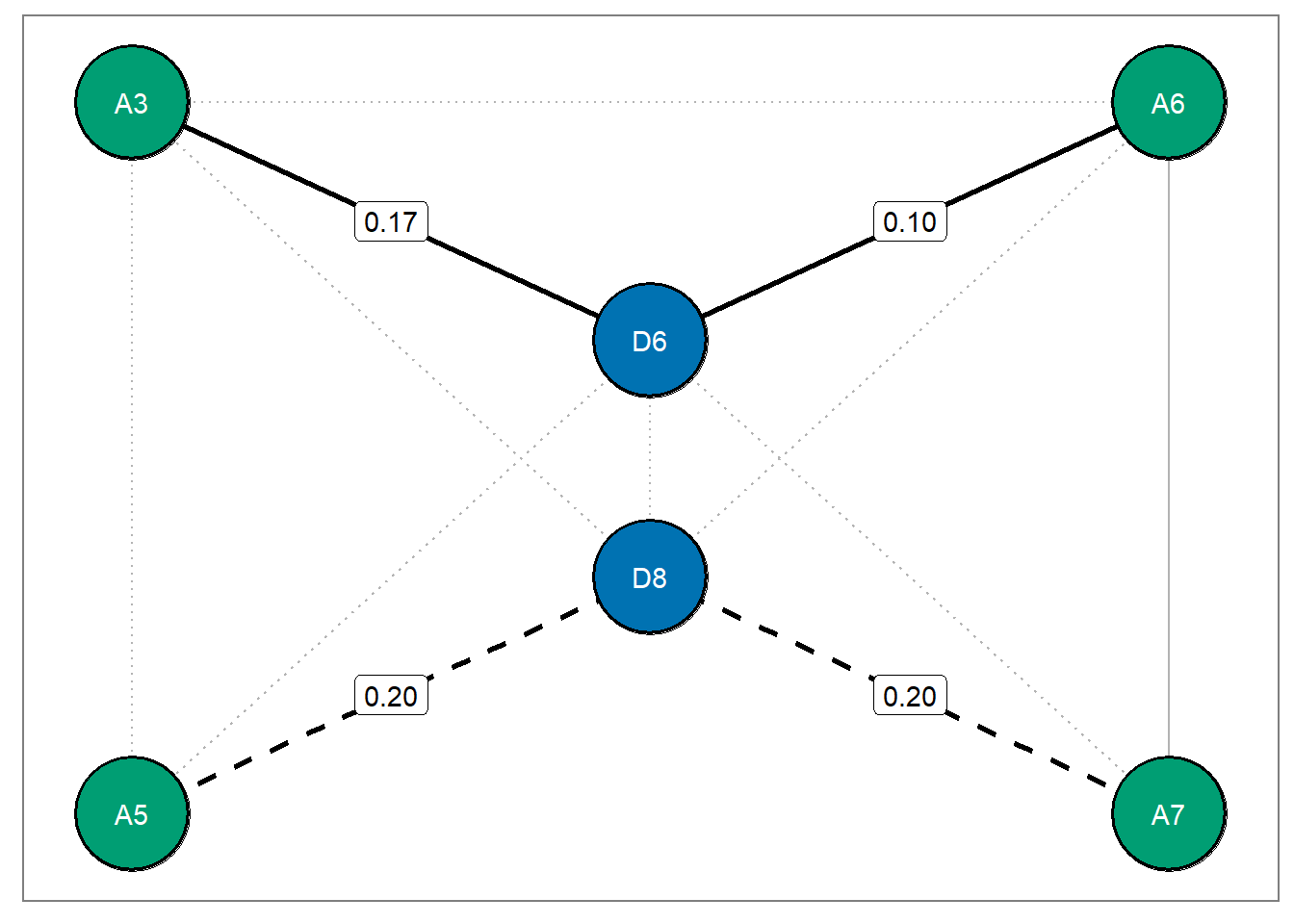
The following hypotheses focus on characterizing bridge sets, or the set of bridge edges belonging to a given symptom. For example, \(\mathcal{H}_1\) posits that the bridge set for node D8 is collectively greater than the set for node D6, with the constraint that the edges within the bridge set for D8 are equal to each other. This effectively corresponds to testing whether node D8 has greater bridge strength than node D6. \(\mathcal{H}_2\) then refines \(\mathcal{H}_1\) by testing an exact order both between and within bridge sets.
\[\begin{align} \label{eq:intra-inter} \mathcal{H}_1 &: \rho_{D8-A5} = \rho_{D8-A7} > (\rho_{D6-A3}, \rho_{D6-A6}) > 0 \\ \nonumber \mathcal{H}_2 &: \rho_{D8-A5} > \rho_{D8-A7} > \rho_{D6-A3} > \rho_{D6-A6} > 0 \\ \nonumber \mathcal{H}_3 &: ``\text{not}\; \mathcal{H}_1 \; \text{or}\; \mathcal{H}_2 \text{.''} \end{align}\]
Note that the inclusion of an inequality and equality constraint in a single hypothesis is currently only available on the GitHub version for BGGM.
intra_inter_hyp <- c("D8--A5 = D8--A7 > (D6--A3, D6--A6) > 0;
                      D8--A5 > D8--A7 > D6--A3 > D6--A6 > 0")

confirm_intra_inter <- confirm(Y = confirm_anxdep,
                               hypothesis = intra_inter_hyp,
                               iter = 50000)
confirm_intra_inter
## BGGM: Bayesian Gaussian Graphical Models
## Type: continuous
## ---
## Posterior Samples: 50000
## Observations (n): 515
## Variables (p): 16
## Delta: 15
## ---
## Call:
## confirm(Y = confirm_anxdep, hypothesis = intra_inter_hyp, iter = 50000)
## ---
## Hypotheses:
##
## H1: D8--A5=D8--A7>(D6--A3,D6--A6)>0
## H2:
## D8--A5>D8--A7>D6--A3>D6--A6>0
## H3: complement
## ---
## Posterior prob:
##
## p(H1|data) = 0.037
## p(H2|data) = 0.954
## p(H3|data) = 0.009
## ---
## Bayes factor matrix:
## H1 H2 H3
## H1 1.000 0.039 4.251
## H2 25.905 1.000 110.115
## H3 0.235 0.009 1.000
## ---
## note: equal hypothesis prior probabilitiesThe data were more likely under both \(\mathcal{H}_1\) (\(\text{BF}_{13} = 4.3\)) and \(\mathcal{H}_2\) (\(\text{BF}_{23} = 110.1\)) than \(\mathcal{H}_3\). Furthermore, there was more evidence supporting the hypothesis testing solely inequality constraints, \(\mathcal{H}_2\), than the one including an equality constraint (\(\text{BF}_{21} = 25.9\)). This provides a clear characterization of the the bridge relations at hand — not only did the order of bridge strength replicate, but so did the order of the edges within each bridge set.
Bridge Set Separation
We also thought it would be interesting to test whether bridge sets include common elements. That is, whether bridge symptoms connect to the same or different nodes. As can be seen above, the bridge sets for nodes D8 and D6 are mutually exclusive. We can then test, say, whether D8 is conditionally independent from the bridge set for D6 (nodes A3 and A6)
\[\begin{align} \mathcal{H}_1 &: (\rho_{D8-A3}, \rho_{D8-A6}) = 0 \\ \nonumber \mathcal{H}_2 &: (\rho_{D8-A3}, \rho_{D8-A6}) > 0 \\ \nonumber \mathcal{H}_3 &: ``\text{not}\; \mathcal{H}_1 \; \text{or} \; \mathcal{H}_2 \text{.''} \end{align}\]
hyp_bridge_sep <- ("(D8--A3, D8--A6) = 0;
                    (D8--A3, D8--A6) > 0")

confirm_bridge_sep <- confirm(Y = confirm_anxdep,
                              hypothesis = hyp_bridge_sep,
                              iter = 50000)
confirm_bridge_sep
## BGGM: Bayesian Gaussian Graphical Models
## Type: continuous
## ---
## Posterior Samples: 50000
## Observations (n): 515
## Variables (p): 16
## Delta: 15
## ---
## Call:
## confirm(Y = confirm_anxdep, hypothesis = hyp_bridge_sep, iter = 50000)
## ---
## Hypotheses:
##
## H1: (D8--A3,D8--A6)=0
## H2:
## (D8--A3,D8--A6)>0
## H3: complement
## ---
## Posterior prob:
##
## p(H1|data) = 0.307
## p(H2|data) = 0.61
## p(H3|data) = 0.084
## ---
## Bayes factor matrix:
## H1 H2 H3
## H1 1.000 0.503 3.665
## H2 1.989 1.000 7.288
## H3 0.273 0.137 1.000
## ---
## note: equal hypothesis prior probabilitiesAlthough the data were more likely under \(\mathcal{H}_1\) than \(\mathcal{H}_3\) (\(\text{BF}_{13} = 3.7\)), there was support in favor of \(\mathcal{H}_2\) compared to \(\mathcal{H}_1\) (\(\text{BF}_{21} = 2\)). This analysis suggests it is unlikely that D8 is actually conditionally independent from the bridge set for D6.
Summary
In this tutorial, I briefly described a framework to formulate and test hypotheses on psychological networks using BGGM. The idea is to (1) identify central structures on which you can formulate hypotheses in an exploratory analysis and (2) test those hypotheses on independent data. This brings networks to fruition as tools to generate hypotheses and overcomes the idea that they are solely for exploratory purposes.
In writing the above paper, our hope is that researchers can integrate these methods into their work. We believe that conducting confirmatory tests is an important step forward in psychological networks.
References
Beard, C., Millner, A. J., Forgeard, M. J. C., Fried, E. I., Hsu, K. J., Treadway, M. T., Leonard, C. V., Kertz, S. J., & Björgvinsson, T. (2016). Network analysis of depression and anxiety symptom relationships in a psychiatric sample. Psychological Medicine, 46(16), 3359–3369. https://doi.org/10.1017/S0033291716002300
Fried, E. I., Eidhof, M. B., Palic, S., Costantini, G., Huisman-van Dijk, H. M., Bockting, C. L. H., Engelhard, I., Armour, C., Nielsen, A. B. S., & Karstoft, K.-I. (2018). Replicability and Generalizability of Posttraumatic Stress Disorder (PTSD) Networks: A Cross-Cultural Multisite Study of PTSD Symptoms in Four Trauma Patient Samples. Clinical Psychological Science, 6(3), 335–351. https://doi.org/10.1177/2167702617745092